System modelling using Z trasform

Transfer function model

Let us assume a discrete SISO discrete system: 

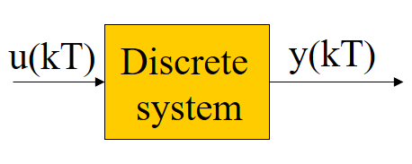
Its  dynamics is described by means of difference equations. For a n-th order linear time invariant system (LTI) the model is

In control engineering, alternative models are used instead of difference equations. The most common model is the transfer function. For a discrete-time syste,  the discrete transfer function is defined as the relation between the ouput Z-transform (Y(z)) and the input Z-transform (U(z)) assuming zero initial conditions:

where  is a complex variable. As commented, the relation between the s-plane and z-plane is  

The dynamics of the system will be defined by its poles location. The poles are obtained as the roots of the denominator of G(z).

State variables

As an alternative to transfer function the state variables model can be defined. State variables are defined as the minimum set of variables so that for a given initial condition, the knowledge of these variables and the future input to be applied is anough to determine the future evolution of the system. 

The state variable model can be expressed using two equations: the state equation (that account for the dynamics of the system) and the output equation (that relates the state varaible to the output variable). Thus, the model is

State equation

(n  first-order difference equation)

Ouput equation

(y is obtained as a linear combination of  x and u)

Stability

The stability of a discrete system can be analyzed from the pole location:

• A discrete system is stable if all its poles falls inside the unit circle.
• A discrete system is unstable if at least one of its poles falls outside the unit circle.